Jupyter Notebooks
Acknowledgements
The material in this tutorial is specific to PYNQ. Wherever possible, however, it re-uses generic documentation describing Jupyter notebooks. In particular, we have re-used content from the following example notebooks:
- What is the Jupyter Notebook?
- Notebook Basics
- Running Code
- Markdown Cells
The original notebooks and further example notebooks are available at Jupyter documentation.
Introduction
If you are reading this documentation from the webpage, you should note that the webpage is a static html version of the notebook from which it was generated. If the PYNQ platform is available, you can open this notebook from the getting_started folder in the PYNQ Jupyter landing page.
The Jupyter Notebook is an interactive computing environment that enables users to author notebook documents that include:
- Live code
- Interactive widgets
- Plots
- Narrative text
- Equations
- Images
- Video
These documents provide a complete and self-contained record of a computation that can be converted to various formats and shared with others electronically, using version control systems (like git/GitHub) or nbviewer.jupyter.org.
Components
The Jupyter Notebook combines three components:
- The notebook web application: An interactive web application for writing and running code interactively and authoring notebook documents.
- Kernels: Separate processes started by the notebook web application that runs users’ code in a given language and returns output back to the notebook web application. The kernel also handles things like computations for interactive widgets, tab completion and introspection.
- Notebook documents: Self-contained documents that contain a representation of all content in the notebook web application, including inputs and outputs of the computations, narrative text, equations, images, and rich media representations of objects. Each notebook document has its own kernel.
Notebook web application
The notebook web application enables users to:
- Edit code in the browser, with automatic syntax highlighting, indentation, and tab completion/introspection.
- Run code from the browser, with the results of computations attached to the code which generated them.
- See the results of computations with rich media representations, such as HTML, LaTeX, PNG, SVG, PDF, etc.
- Create and use interactive JavaScript widgets, which bind interactive user interface controls and visualizations to reactive kernel side computations.
- Author narrative text using the Markdown markup language.
- Build hierarchical documents that are organized into sections with different levels of headings.
- Include mathematical equations using LaTeX syntax in Markdown, which are rendered in-browser by MathJax.
Kernels
The Notebook supports a range of different programming languages. For each notebook that a user opens, the web application starts a kernel that runs the code for that notebook. Each kernel is capable of running code in a single programming language. There are kernels available in the following languages:
- Python https://github.com/ipython/ipython
- Julia https://github.com/JuliaLang/IJulia.jl
- R https://github.com/takluyver/IRkernel
- Ruby https://github.com/minrk/iruby
- Haskell https://github.com/gibiansky/IHaskell
- Scala https://github.com/Bridgewater/scala-notebook
- node.js https://gist.github.com/Carreau/4279371
- Go https://github.com/takluyver/igo
PYNQ is written in Python, which is the default kernel for Jupyter Notebook, and the only kernel installed for Jupyter Notebook in the PYNQ distribution.
Kernels communicate with the notebook web application and web browser using a JSON over ZeroMQ/WebSockets message protocol that is described here. Most users don’t need to know about these details, but its important to understand that kernels run on Zynq, while the web browser serves up an interface to that kernel.
Notebook Documents
Notebook documents contain the inputs and outputs of an interactive session as well as narrative text that accompanies the code but is not meant for execution. Rich output generated by running code, including HTML, images, video, and plots, is embedded in the notebook, which makes it a complete and self-contained record of a computation.
When you run the notebook web application on your computer, notebook documents are just files on your local filesystem with a .ipynb extension. This allows you to use familiar workflows for organizing your notebooks into folders and sharing them with others.
Notebooks consist of a linear sequence of cells. There are four basic cell types:
- Code cells: Input and output of live code that is run in the kernel
- Markdown cells: Narrative text with embedded LaTeX equations
- Heading cells: Deprecated. Headings are supported in Markdown cells
- Raw cells: Unformatted text that is included, without modification, when notebooks are converted to different formats using nbconvert
Internally, notebook documents are JSON data with binary values base64 encoded. This allows them to be read and manipulated programmatically by any programming language. Because JSON is a text format, notebook documents are version control friendly.
Notebooks can be exported to different static formats including
HTML, reStructeredText, LaTeX, PDF, and slide shows
(reveal.js) using Jupyter’s
nbconvert utility. Some of documentation for Pynq, including this
page, was written in a Notebook and converted to html for hosting on the
project’s documentation website.
Furthermore, any notebook document available from a public URL or on GitHub can be shared via nbviewer. This service loads the notebook document from the URL and renders it as a static web page. The resulting web page may thus be shared with others without their needing to install the Jupyter Notebook.
GitHub also renders notebooks, so any Notebook added to GitHub can be viewed as intended.
Notebook Basics
The Notebook dashboard
The Notebook server runs on the ARM® processor of the PYNQ-Z1. You can open the notebook dashboard by navigating to pynq:9090 when your board is connected to the network. The dashboard serves as a home page for notebooks. Its main purpose is to display the notebooks and files in the current directory. For example, here is a screenshot of the dashboard page for an example directory:
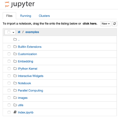
The top of the notebook list displays clickable breadcrumbs of the current directory. By clicking on these breadcrumbs or on sub-directories in the notebook list, you can navigate your filesystem.
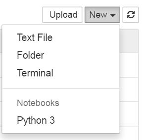
To create a new notebook, click on the “New” button at the top of the list and select a kernel from the dropdown (as seen below).
Notebooks and files can be uploaded to the current directory by dragging a notebook file onto the notebook list or by the “click here” text above the list.
The notebook list shows green “Running” text and a green notebook icon next to running notebooks (as seen below). Notebooks remain running until you explicitly shut them down; closing the notebook’s page is not sufficient.

To shutdown, delete, duplicate, or rename a notebook check the checkbox next to it and an array of controls will appear at the top of the notebook list (as seen below). You can also use the same operations on directories and files when applicable.

To see all of your running notebooks along with their directories, click on the “Running” tab:
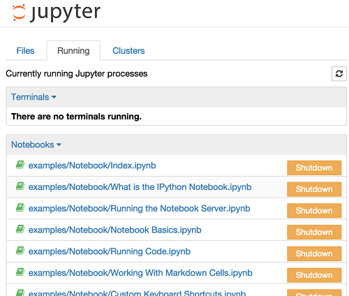
This view provides a convenient way to track notebooks that you start as you navigate the file system in a long running notebook server.
Overview of the Notebook UI
If you create a new notebook or open an existing one, you will be taken to the notebook user interface (UI). This UI allows you to run code and author notebook documents interactively. The notebook UI has the following main areas:
- Menu
- Toolbar
- Notebook area and cells
The notebook has an interactive tour of these elements that can be started in the “Help:User Interface Tour” menu item.
Modal editor
The Jupyter Notebook has a modal user interface which means that the keyboard does different things depending on which mode the Notebook is in. There are two modes: edit mode and command mode.
Edit mode
Edit mode is indicated by a green cell border and a prompt showing in the editor area:

When a cell is in edit mode, you can type into the cell, like a normal text editor.
Enter edit mode by pressing Enter or using the mouse to click on a
cell’s editor area.
Command mode
Command mode is indicated by a grey cell border with a blue left margin:

When you are in command mode, you are able to edit the notebook as a
whole, but not type into individual cells. Most importantly, in command
mode, the keyboard is mapped to a set of shortcuts that let you perform
notebook and cell actions efficiently. For example, if you are in
command mode and you press c, you will copy the current cell - no
modifier is needed.
Don’t try to type into a cell in command mode; unexpected things will happen!
Enter command mode by pressing Esc or using the mouse to click
outside a cell’s editor area.
Mouse navigation
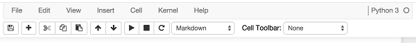
All navigation and actions in the Notebook are available using the mouse through the menubar and toolbar, both of which are above the main Notebook area:
Cells can be selected by clicking on them with the mouse. The currently selected cell gets a grey or green border depending on whether the notebook is in edit or command mode. If you click inside a cell’s editor area, you will enter edit mode. If you click on the prompt or output area of a cell you will enter command mode.
If you are running this notebook in a live session on the PYNQ-Z1, try selecting different cells and going between edit and command mode. Try typing into a cell.
If you want to run the code in a cell, you would select it and click the
play button in the toolbar, the “Cell:Run” menu item, or type Ctrl +
Enter. Similarly, to copy a cell you would select it and click the
copy button in the toolbar or the “Edit:Copy” menu item. Ctrl + C, V
are also supported.
Markdown and heading cells have one other state that can be modified
with the mouse. These cells can either be rendered or unrendered. When
they are rendered, you will see a nice formatted representation of the
cell’s contents. When they are unrendered, you will see the raw text
source of the cell. To render the selected cell with the mouse, and
execute it. (Click the play button in the toolbar or the “Cell:Run”
menu item, or type Ctrl + Enter. To unrender the selected cell, double
click on the cell.
Running Code
First and foremost, the Jupyter Notebook is an interactive environment for writing and running code. The notebook is capable of running code in a wide range of languages. However, each notebook is associated with a single kernel. Pynq, and this notebook is associated with the IPython kernel, which runs Python code.
Code cells allow you to enter and run code
Run a code cell using Shift-Enter or pressing the play button in
the toolbar above. The button displays run cell, select below when you
hover over it.
In [1]:
a = 10
In [ ]:
print(a)
There are two other keyboard shortcuts for running code:
Alt-Enterruns the current cell and inserts a new one below.Ctrl-Enterrun the current cell and enters command mode.
Managing the Kernel
Code is run in a separate process called the Kernel. The Kernel can be
interrupted or restarted. Try running the following cell and then hit
the stop button in the toolbar above. The button displays interrupt
kernel when you hover over it.
In [ ]:
import time
time.sleep(10)
Restarting the kernels
The kernel maintains the state of a notebook’s computations. You can reset this state by restarting the kernel. This is done from the menu bar, or by clicking on the corresponding button in the toolbar.
sys.stdout
The stdout and stderr streams are displayed as text in the output area.
In [ ]:
print("Hello from Pynq!")
Output is asynchronous
All output is displayed asynchronously as it is generated in the Kernel. If you execute the next cell, you will see the output one piece at a time, not all at the end.
In [ ]:
import time, sys
for i in range(8):
    print(i)
    time.sleep(0.5)
Large outputs
To better handle large outputs, the output area can be collapsed. Run the following cell and then single- or double- click on the active area to the left of the output:
In [ ]:
for i in range(50):
    print(i)
Markdown
Text can be added to Jupyter Notebooks using Markdown cells. Markdown is a popular markup language that is a superset of HTML. Its specification can be found here:
http://daringfireball.net/projects/markdown/
Markdown basics
You can make text italic or bold.
You can build nested itemized or enumerated lists:
- One
- Sublist
- This
- Sublist
- Sublist - That - The other thing
- Two
- Sublist
- Three
- Sublist
Now another list:
- Here we go
- Sublist
- Sublist
- There we go
- Now this
You can add horizontal rules:
Here is a blockquote:
Beautiful is better than ugly. Explicit is better than implicit. Simple is better than complex. Complex is better than complicated. Flat is better than nested. Sparse is better than dense. Readability counts. Special cases aren’t special enough to break the rules. Although practicality beats purity. Errors should never pass silently. Unless explicitly silenced. In the face of ambiguity, refuse the temptation to guess. There should be one– and preferably only one –obvious way to do it. Although that way may not be obvious at first unless you’re Dutch. Now is better than never. Although never is often better than right now. If the implementation is hard to explain, it’s a bad idea. If the implementation is easy to explain, it may be a good idea. Namespaces are one honking great idea – let’s do more of those!
And shorthand for links:
Headings
You can add headings by starting a line with one (or multiple) #
followed by a space, as in the following example:
# Heading 1
# Heading 2
## Heading 2.1
## Heading 2.2
Embedded code
You can embed code meant for illustration instead of execution in Python:
def f(x):
    """a docstring"""
    return x**2
or other languages:
if (i=0; i<n; i++) {
  printf("hello %d\n", i);
  x += 4;
}
LaTeX equations
Courtesy of MathJax, you can include mathematical expressions inline or displayed on their own line.
Inline expressions can be added by surrounding the latex code with
$:
Inline example: $e^{i\pi} + 1 = 0$
This renders as:
Inline example: \(e^{i\pi} + 1 = 0\)
Expressions displayed on their own line are surrounded by $$:
$$e^x=\sum_{i=0}^\infty \frac{1}{i!}x^i$$
This renders as:
GitHub flavored markdown
The Notebook webapp supports Github flavored markdown meaning that you can use triple backticks for code blocks:
<pre>
```python
print "Hello World"
```
</pre>

<pre>
```javascript
console.log("Hello World")
```
</pre>
Gives:
print "Hello World"
console.log("Hello World")
And a table like this:
<pre>
```

| This | is   |
|------|------|
|   a  | table|

```
</pre>
A nice HTML Table:
| This | is |
|---|---|
| a | table |
General HTML
Because Markdown is a superset of HTML you can even add things like HTML tables:
Header 1 | Header 2 |
|---|---|
row 1, cell 1 | row 1, cell 2 |
row 2, cell 1 | row 2, cell 2 |
Local files
If you have local files in your Notebook directory, you can refer to these files in Markdown cells directly:
[subdirectory/]<filename>
Security of local files
Note that the Jupyter notebook server also acts as a generic file server for files inside the same tree as your notebooks. Access is not granted outside the notebook folder so you have strict control over what files are visible, but for this reason it is highly recommended that you do not run the notebook server with a notebook directory at a high level in your filesystem (e.g. your home directory).
When you run the notebook in a password-protected manner, local file access is restricted to authenticated users unless read-only views are active. For more information, see Jupyter’s documentation on running a notebook server.